Last time we talked about different options for validating data in Google Sheets. You’ve already learned how to create simple drop-down lists using Data Validation. Today, we’re going to dive deeper. You’ll discover how to build business metrics monitors using Data Validation, the FILTER formula, and dependent drop-down lists. Also, you’ll learn a few formatting tips and tricks.

If you prefer watching to reading, check out the YouTube version of this tutorial.

Why you need data filtering

When you need to filter data in Google Sheets, it means you have to set rules to display certain information. This function is rather useful when you work with large datasets. Filtering lets you focus on relevant data and increase your performance.

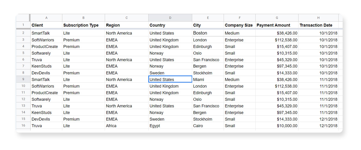
That’s it for the boring theory stuff. Let’s try hands-on. For this, you can get a personal copy of the Google Sheets practice file with Data Validation task for exercising. As a dataset, we’ll use the payments database we often use in other Google Sheets videos.

How to create an income monitor

Imagine you want to have an income monitor based on the locations. There are clients from different regions, countries, and cities. You need the results to change depending on the exact location you select.

Moreover, you can connect the income monitor to your CRM app and get it updated automatically using Coupler.io. Check out the blog post, How to Build Sales Tracker with Google Sheets, to learn details.

Dynamic drop-down lists

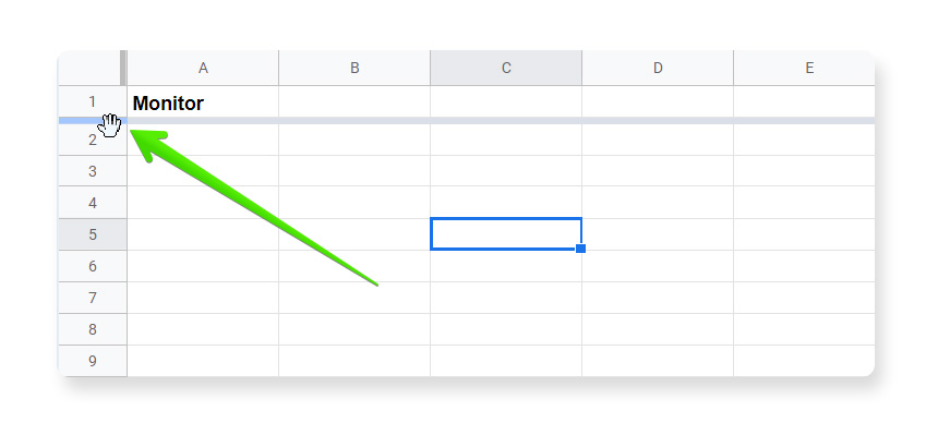
First, create a dynamic drop-down list. For this, get a separate tab called “Income Monitor”. We recommend you store data sources and calculations on separate tabs. Now, mark the monitor and freeze the first row, as it will contain headers. You can do this by pulling the marker.

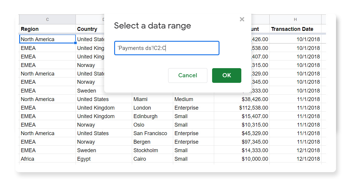
Then, mark where you’ll have Region, Country, and City in the monitor. Now, let’s apply the standard data validation to the region. To do this, click on the cell next to it, use Control+Option+D (Ctrl+Alt+D for Windows) and then press V. Or you may right-click on the cell and select Data Validation in the bottom of the list. In the menu, set the List from a range criteria and select the Regions column in the Payments Tab. Don’t forget to specify the whole column in the Select a data range box, so that you don’t miss anything when the new data is entered. For this, enter ‘Payments’!C2:C.

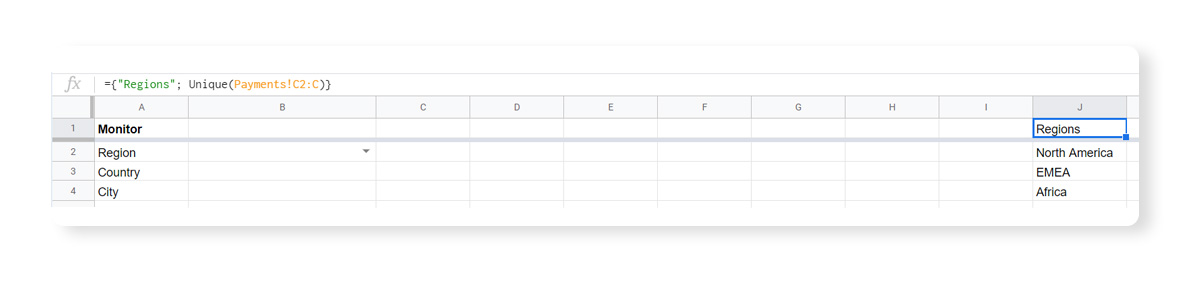
Google Sheets automatically pulls unique values to the dropdown list, so that you don’t see duplicates. Here is what you should get in your Income Monitor tab.

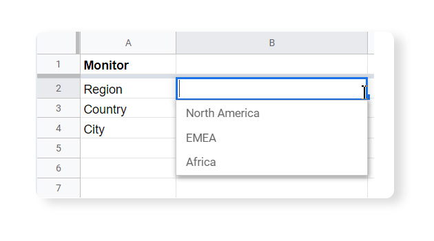
Also, let’s pull unique regions to the list on the right, so it will be visible. It will be easier to validate the region based on the list in the same tab. So, let’s use these values for data validation in the monitor.

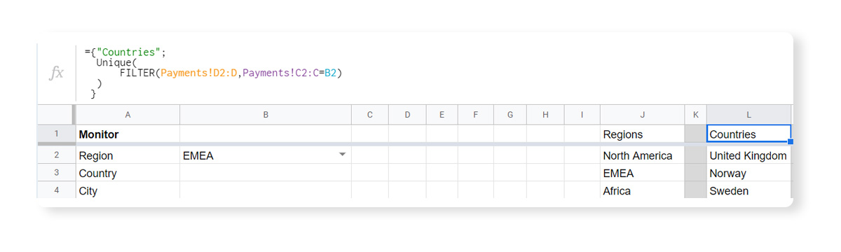
Select a cell and use braces to add a header right in the formula. Start from the header and then write down the formula:
={"Regions";
Unique(Payments!C2:C)}

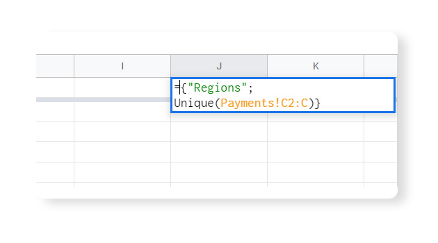
The unique formula pulls unique values from the Regions column in the Payments tab. You may split the formula into few lines to make it more readable. Press Enter.

Dependent drop-down lists

It will be easier to see the list of cities only from the selected regions and countries. Besides, you won’t have to remind yourself whether Bergen is in Sweden or Norway every time. So let’s use the dependent drop-down lists.

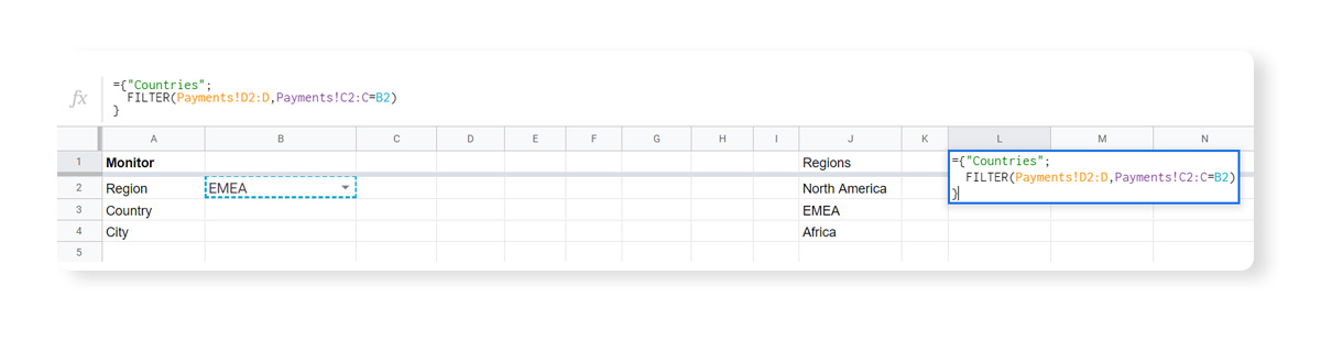
For this, you need to create a few helpers. First, use the Filter formula to list the countries from the selected region. You can learn more about how to use Filter formulas in our tutorial. Select a cell and write down:
={"Countries";
FILTER(Payments!D2:D,Payments!C2:C=B2)
}

"Countries" refers to the header.
Payments!D2:D denotes the range to filter (the countries column in the Payments tab).
Payments!C2:C=B2 denotes the criteria to match (the region column in Payments) to match the region selected in the monitor.
FILTER(Payments!D2:D,Payments!C2:C=B2) refers to filtering the countries where the region is equal to the one selected in our monitor.
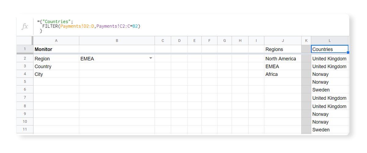
Make sure you’ve formatted your formula and hit Enter.

Ok, so now you have the whole list of countries from the selected region filtered out here.

To get rid of the duplicates, you can apply UNIQUE. Wrap the FILTER in parents and put UNIQUE before it. This will pull the unique values from the filtered list.

={"Countries";
Unique(
FILTER(Payments!D2:D,Payments!C2:C=B2)
)
}

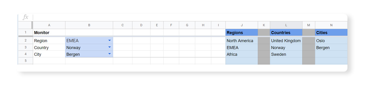
Now, if you select a different region, the countries list will change as well.

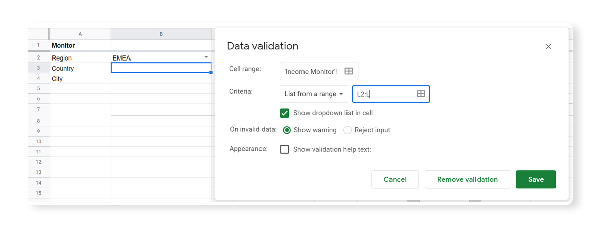
Let’s apply data validation to the Country in our monitor. Control+Option+D (Ctrl+Alt+D for Windows), then V, or right-click on the cell and select Data Validation in the bottom of the list. As a data range, we select Countries (L2:L).

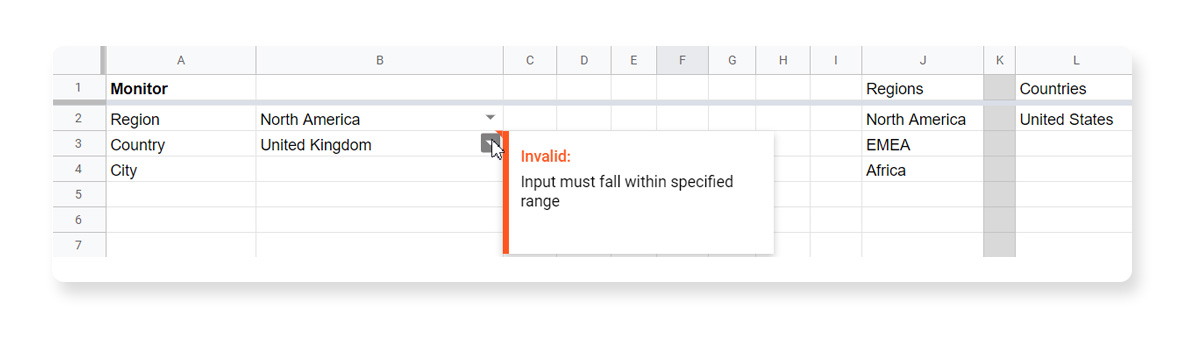
Now, if the region changes, the country might get marked as invalid.

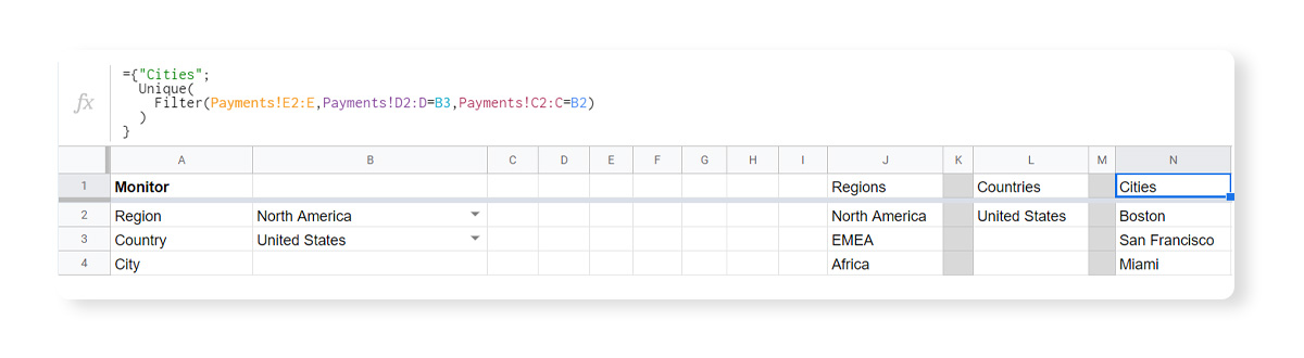
Do the same to validate City. But here you need two conditions in the FILTER formula – for both Region and Country to match. So add one more condition.

={"Cities";
Unique(
FILTER(Payments!E2:E,Payments!D2:D=B3,Payments!C2:C=B2)
)
}

Payments!E2:E – set to filter
Payments!D2:D=B3 – Countries to match the one in the monitor
Payments!C2:C=B2 – Region to match the one in the monitor

Hit enter.

If for some reason, Region and Country don’t match, the Cities list won’t show. It may happen when you change Region but not Country. This is an additional reminder for you to select the matching region and country.

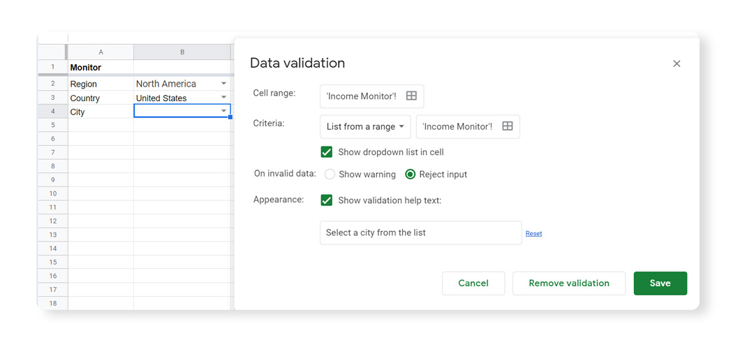
Now, add the Cities range as a criteria to validate City in our monitor. Perform the regular operation to apply data validation and select a data range (N2:N). You can also mark Reject input on invalid data and add a note (mark Show validation help text) “Select a city from the list”.

Color coding to format a spreadsheet

If you want to visually mark the structure, color coding can help you with this. It is also very helpful when multiple users work with your spreadsheet. You can color the cells with formulas, as well as the cells with dynamic data, to make sure nobody re-writes them.

Use different colors for outputs and calculations. You can also delete the unneeded rows. To make datasets visually independent from each other, add color boundaries between them (like in columns K and M).

Calculating income

Now, it’s time to calculate values you want to see. As an example, let’s find out the total income from the clients in a particular city. This will be Bergen.

• Use SUM(FILTER
• Select the Payment Amount column from the datasource to be filtered – Payments!G2:G
• Select criteria to match the values above
  • Region in the datasource to match the Region selected in the monitor – Payments!C2:C=B2
  • Country in the datasource to match the Country selected in the monitor – Payments!D2:D=B3
  • City in the datasource to match the City selected in the monitor – Payments!E2:E=B4

You should get the following:
=SUM(
Filter(Payments!G2:G,Payments!C2:C=B2,Payments!D2:D=B3,Payments!E2:E=B4)
)

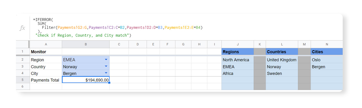
To trap and manage errors, apply IFERROR formula to the Filter. If an error occurs, add a message “Check if Region, Country, and City match”. Here how it looks:

=IFERROR(
SUM(
Filter(Payments!G2:G,Payments!C2:C=B2,Payments!D2:D=B3,Payments!E2:E=B4)
),
"check if Region, Country, and City match")

And here it is – the sum of the payments based on the multiple criteria.

You can apply this approach to different contexts:

• to see the list of clients in the region
• to track unpaid invoices, etc.

   

  Using other formulas, like FILTER, provides more capabilities to track data. FILTER lets you pull information about clients and their payments based on the Region, Country, and City you select. For this:

  • add headers first – open braces and pull all the headers from the datasource (from A1 to H1) – =Payments!A1:H1;
  • type IFERROR(FILTER( and specify values from A2:H and the filter criteria (Region, Country, and City) to match the values from the monitor – Payments!A2:H,Payments!C2:C=B2,Payments!D2:D=B3,Payments!E2:E=B4

  Here how it looks:
  ={Payments!A1:H1;
IFERROR(
Filter(Payments!A2:H,Payments!C2:C=B2,Payments!D2:D=B3,Payments!E2:E=B4)
)
}

  If all criteria match, you’ll see a list of payments from different clients.

  

  If criteria don’t match, the list will be empty. You can discover more tips and tricks with Filter formula in our video.

  That’s it, you income monitor is ready to use. Google Sheets still has many quirks, and the Railsware team will be demystifying them for its readers and viewers in upcoming posts. So, read our blog and subscribe to our YouTube channel to get more interesting insights.