Google Sheets is a powerful tool you can use for a variety of data-driven tasks. At the same time, to get into the intricacies GSheets can provide, you need to start from the basics. And this tutorial for beginners is meant to help you with that. Here we go!

Before we begin, make sure that you have an active Google account. If you don’t have one, we do recommend you spend a few minutes to create it. The tutorial will be more useful if you reconcile theory and practice right away. If you prefer watching than reading, check out the YouTube version of this tutorial.

How to create and find a spreadsheet in Google Drive

To create a new spreadsheet, go to Google Drive. It contains folders and files, and you need to create a new folder by clicking + New on top. Let’s call it Google Sheets for Beginners. Click Create to proceed.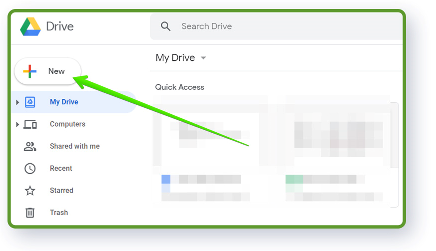

After that you can create a new Google Sheet: Go to folder → Click + New on top → Google Sheets → select whether you want to create a blank sheet or use a template. For templates, you can either create and upload templates specific for your organization, or use Google templates gallery. Let’s pick a blank sheet now.

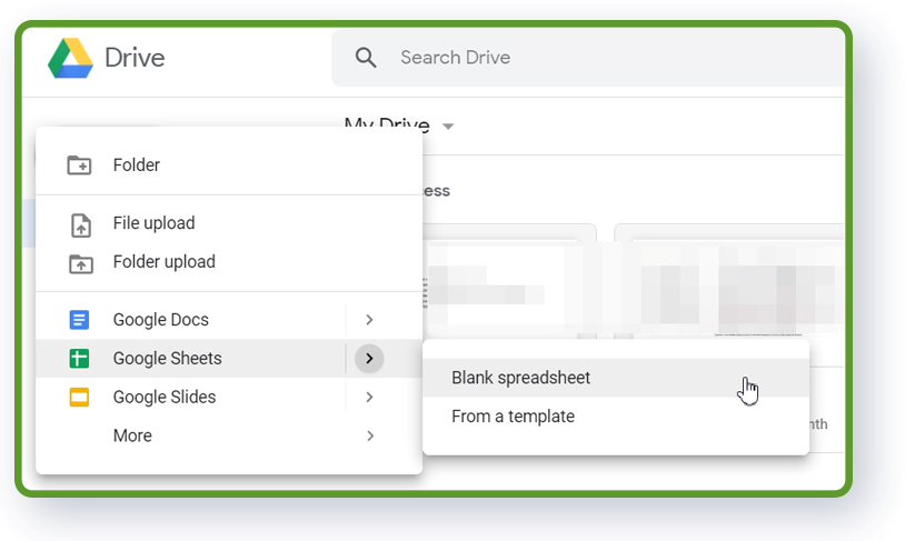
How to create a spreadsheet with sheets.new

One of the coolest tricks with creating a Google spreadsheet is to use .new. Type sheets.new in your browser, and you get a new spreadsheet created right away! It is automatically saved on your Google Drive.

Name the spreadsheet in the top left corner to find it easily next time using search in Google Drive. If you want to organize it, click on the folder icon. Here, you can either create a new folder to store this file or select an existing one.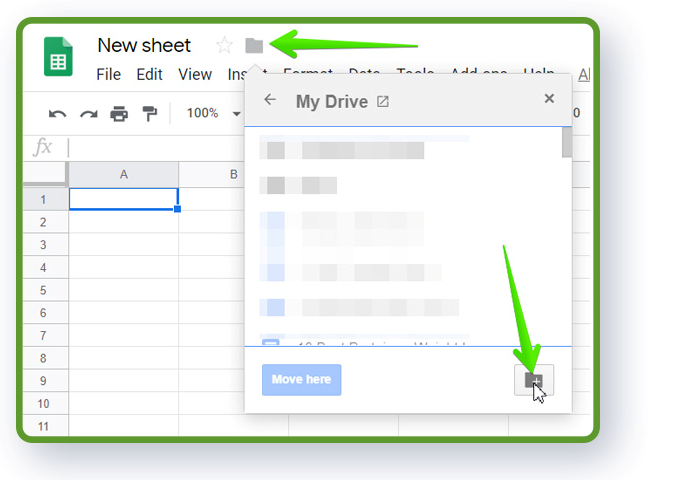

How to upload an existing spreadsheet

You can upload your Excel or CSV file and get it converted into a Google Sheet. For this, you need to drag and drop your file to the folder on Google Drive. For multiple files, go to the Settings menu and select Convert uploaded files to avoid converting each file manually. Now, any file added to GDrive will be automatically converted without copies.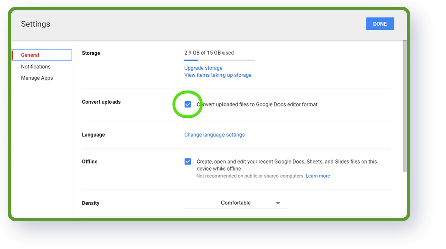

If for some reason, you cannot make edits in your Excel or CSV file after conversion, don’t worry. To make it editable, click Open with Google Sheets on top. Google will create a Google Sheet copy in the same folder.

Working with spreadsheets

Let’s go back to our blank spreadsheet. Keep in mind that Google Drive automatically saves every change you make. This message on top always shows when a change was saved.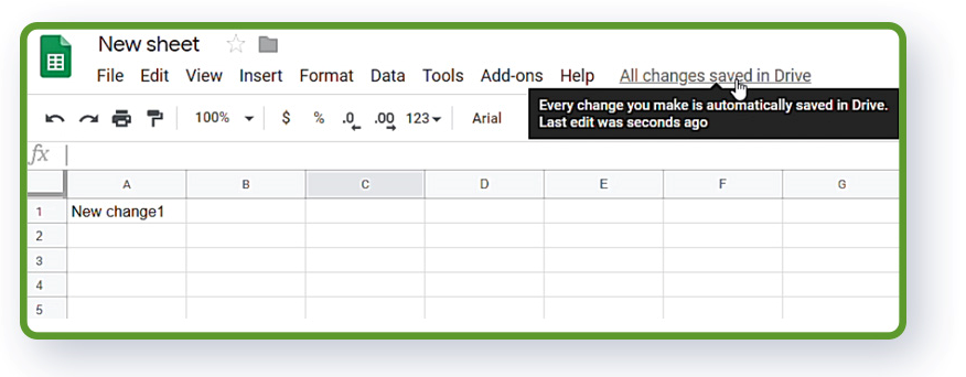

Add, rename, delete, and other manipulations with sheets

One spreadsheet may contain a number of sheets. We advise you to use separate ones to keep your raw data, calculations, and dashboards organized. You can find sheets in the bottom. To rename a sheet, double click on it and type the name you want. To add one more sheet, click the plus, and a new sheet appears.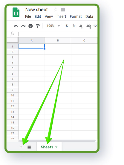

You can change the order by clicking on the sheet, holding and dragging it to the right place. If you right-click on the sheet, you can delete, duplicate, even copy it to another spreadsheet in your Google Drive.

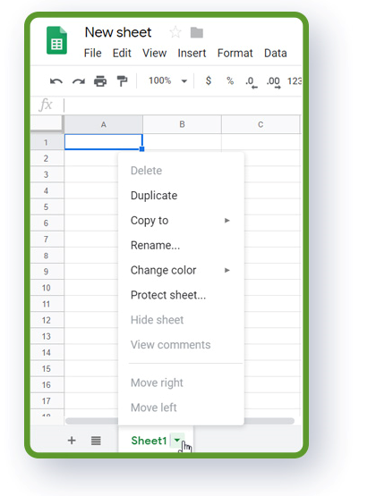You can also change the color of each sheet. Color coding can be very helpful if you have several sheets with raw data and calculations.

If you click All Sheets, you will see the list with color marks, and can navigate through them. This helps a lot in case you have 10 or 20 sheets in the same file, and they get hidden on the right.

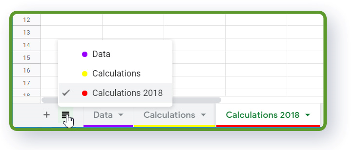
Sheet structure

Each sheet has cells, columns and rows.

Columns and rows

Columns are indicated alphabetically. Rows are indicated numerically.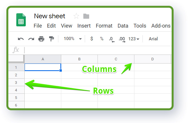

Select the whole column or the whole row by clicking on the index. If you right-click, you can see a list of options to do with a row or column: cut, copy, hide, resize, etc. You can also insert a new column on the left or right. When doing this, remember that the spreadsheet will copy the format of the original column you’ve selected to the newly created one. Similarly, you can insert new rows above or below.

To select the whole sheet, use this button in the top left corner.

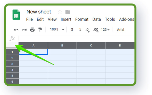You can also freeze columns and rows (keep them visible at any time) with these markers.

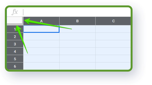
Cells

Cells allow you to both store data and make calculations based on the data in other cells. Each cell has an index – a combination of the column and row indexes. Examples are A1, B2, C3, etc. Indexes are quite useful for selecting different cell ranges.

For example, if you need to sum a specific range of cells, you can select them by clicking the first cell and dragging the entire range. However, if you have a much larger dataset to work with, you can type the cell index where the range starts, colon, and the last cell index. Thus, SUM (E2:E243) means that all the values starting from the cell indexed E2 to the cell indexed E243 will be summed. Here are the most common ways to select different ranges:

• (A2,A5) – to use only the values in A2 and A5. Hold Command (for Mac) or Ctrl (for PC) and click on the cells to select.
• (A2:A5) – to use all values in the cells from A2 to A5. Click on the first cell and drag to select other cells.
• (A:A) – to use all numbers in the column. Simply click on the column index to select it.
• (A3:A) – to use all values from A3 to the end of the column.
• (2:2) – to use values in row #2. Simply click on the row index to select it.
• (A2:2) – to use values from A2 to the end of the row.

Data types

You can input text, numerical information, dates, currencies. To input data in the sheet, click on the cell. You can simply type the data right away or use a field here on the top. You can adjust the size of the field. But don’t forget to select the correct cell before you use this input field. Entering data here is super useful when working with large functions.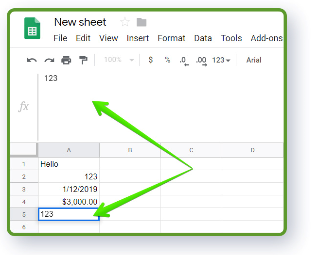

The spreadsheet automatically recognizes the type of data you enter. The text is aligned on the left, numbers and dates – on the right. However, you can adjust the format manually. Use FORMAT to select the type of data you input.

The buttons in the menu allow you to convert numbers into $ or %, as well as decrease or increase decimal places.

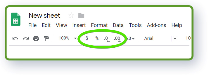
Data formatting

To apply text formatting, you need to select the cells you want and design your texts by using font, text size, bold, italic, strikethrough, text color, etc.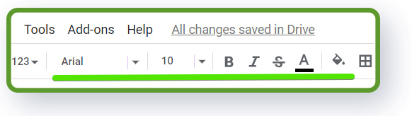

You can manage text wrapping in each cell using this button in the menu. It allows you to overflow, wrap or clip text. Another option is to resize the columns manually.

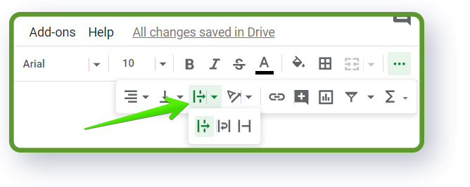If you want to color cells to mark the headers, different types of data, or cells containing formulas and function outcomes, select the cells and use the fill color button.

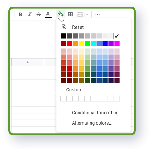You can also add visible borders using this button in the menu. It is helpful in case you want to print the results. Select the cells you want to have visible borders and apply the corresponding option: all the borders, internal borders, one border in the top, bottom, left or right, and so on. The design of your borders (color and style) can be tuned as well.

At the same time, we do not recommend you use the borders. If you move the cell, column or row, the border will move as well. Hence, you will have to reformat your sheet over and over again.

Google Sheets shortcuts

Here are some hotkeys and keyboard functions for you to use when working with spreadsheets.

• To move around the sheet, you can use the keyboard arrows.

• Regular keyboard shortcuts are available with Google Sheets as well:
  Important note: If you copy several cells, the pasted output will contain the same cells in the same order. This might rewrite the data, so make sure you paste into empty cells.
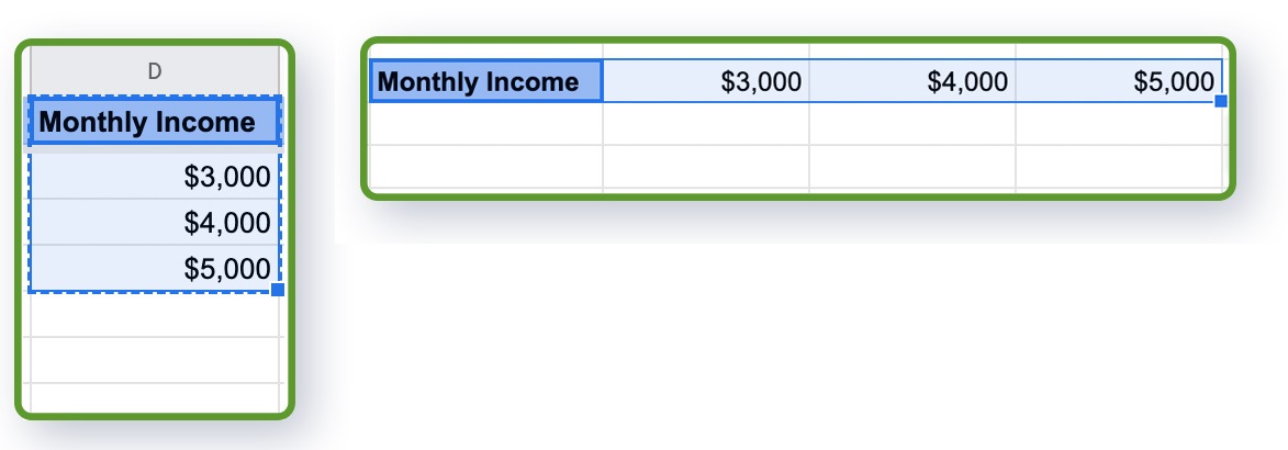
  There are different parts of the data that you can paste once copied. When you copy a set, right-click on the cell and pick Paste special to select what you want to paste: values only, format only and so on.A really cool Google Sheets feature is Paste transposed. It turns the pasted data around: what was in columns will now appear in rows and vice versa.

• There is a hotkey to select a set – Command+Shift+Direction Arrow for Mac/Control+Shift+Direction Arrow for PC.
  
  Click on the cell you want to start from, and press Command/Control+Shift. If you use the right arrow, it will select all of the cells that contain values on the right. If you press it once more, it will select all of the cells in the row. Use the left arrow to select the cells with values only.
  Now, you can press Command/Control+Shift+Down, and Google Sheets will expand the selection to all of the columns in the set. You can select two individual cells by holding the Command key for Mac, or Control key for PC.

Smart Spreadsheets

If you input text and pull the bottom right corner, it will simply copy this text to the next cell. However, spreadsheet is smart. If you input a date, or a day of the week/month, select it, drag, and the sequence will be expanded. The same works for numbers in case you select two of them and drag the bottom right corner of the cell.

Cells allow you to both store data and make calculations based on the data in other cells. To make calculations, use simple math operators in spreadsheets.

For example, you need to count the sum of monthly salaries of your employees. Add a column header first – Salaries Total. Select a cell, type an equals sign, click on the cells with salaries and add a plus between them.

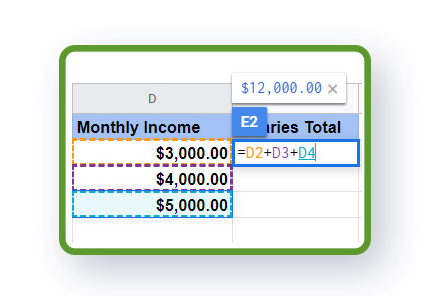You can add numbers manually or refer to the cells with values. Hit Enter and here is the sum of salaries.

If you want to get an average salary, add a column header Salaries Average, type an equals sign, click the cell containing the total value, and divide (/) it by 3.

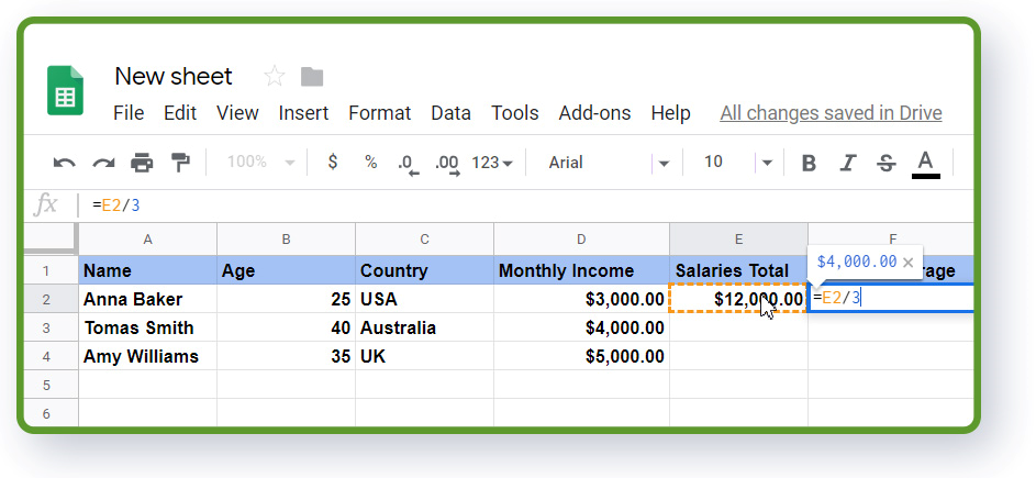If there is a repeatable calculation, and you drag the bottom right corner down, the spreadsheet will extend the calculation using the values in the new rows.

Let’s count the annual salary for our assumed employees. Create a new column, add a header Annual Salary. Now, type an equals sign, refer to the cell with the monthly salary by clicking on it or type its cell index, and multiply it (*) by 12. Press Enter.

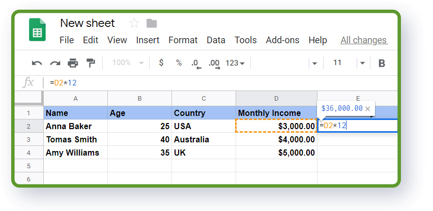If you drag this cell down, it will copy formula for other employees. The annual salary will be calculated differently for each of them based on their monthly income, as the spreadsheet refers to different values for each new row.

Use of data from different sheets

You can refer to cells in the same sheet or in a different sheet. Moreover, you can refer to a totally different spreadsheet from your GDrive. Let’s add the number of months to a separate cell in the Data sheet and refer to it in the formula. Add it to the formula field and hit Enter.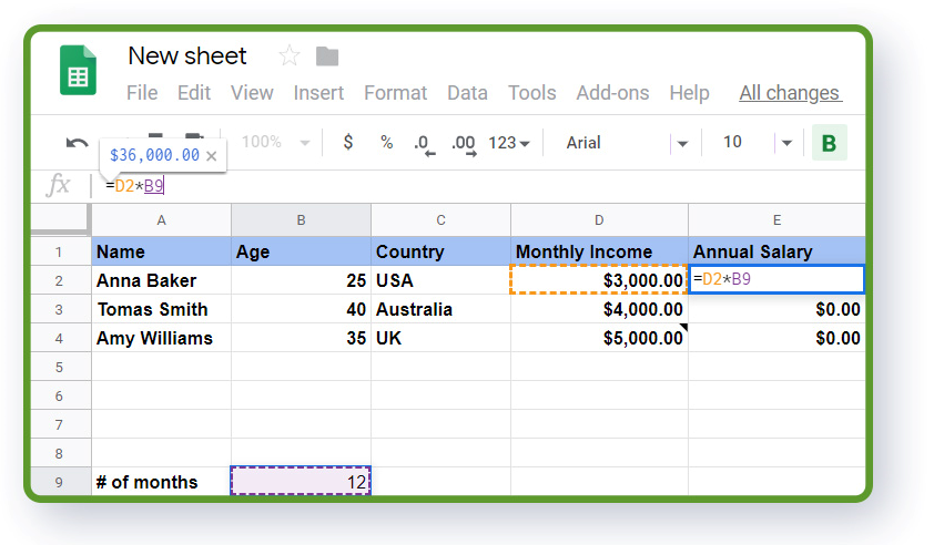

If you drag this formula, it won’t work properly. The months’ number needs to stay the same for all of the copied formulas. For this, you can anchor the values inside the formula using the dollar sign ($). Put $ before the letter to lock this one if formula moves to a new column, and put $ before the number to anchor this value when moving to a different row.

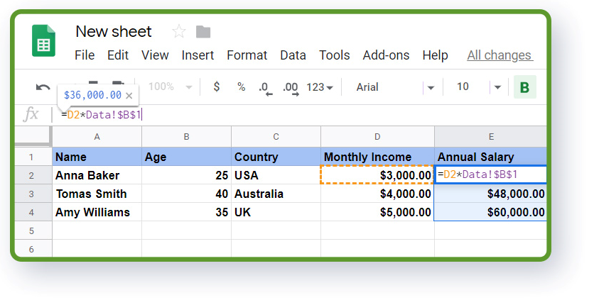In this example, you need to lock the number since the formula is copied to several new rows. After that, if you drag it again, and the formula will work. Use this visual tip until you master the $ anchor in spreadsheets:

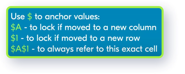
Functions in Google Sheets

One of the most useful features of Google Sheets is using different functions. To use a function, put an equals sign in a cell and start typing the name of the function. Once you do that, the list of possible functions will pop up, and you can choose one of them.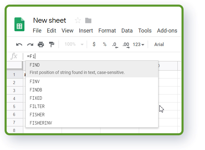

You can find a list of quick functions in the menu as well.

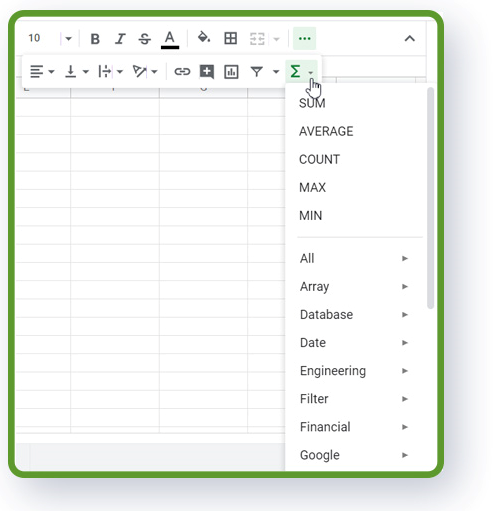Let’s try one of the most common functions – SUM. Click on a new cell, select the function (SUM) and then select the range to be summed (monthly salaries, for example). Hit Enter and get the result! Watch our video about advanced SUM, SUMIF, SUMIFS functions to total values based on a specific criterion.

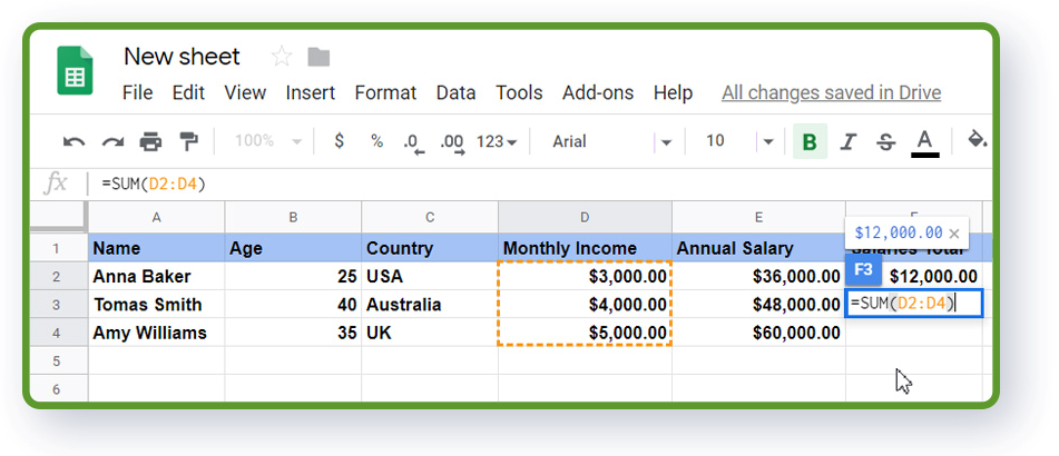Other functions allow you to calculate the average value (=AVERAGE()), count the items in the selected range (=COUNT()), upload data from another spreadsheet (=IMPORTRANGE()), and so on. Follow the same logic: an equals sign, function name, open parentheses, add a range, close parentheses, hit Enter. There is a huge number of functions in Google Sheets. Subscribe to Railsware’s channel to learn the most useful ones.

Collaborate in a spreadsheet using comments and notes

The last but not the least. Google Sheets is a great tool for teams to collaborate on data. There are several features that allow multiple users to work together in one spreadsheet at the same time.

If you work with your teammates on the same document, but not at the same time, you can leave your comments and notes for them. Right-click on the cell, and insert a comment or a note. Notes pop up if you hover over the cell. They are used to add descriptions to the data in the cells. You can leave explanations and hints for your colleagues in notes.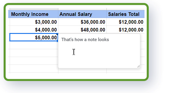

Comments are actionable. You can see who is the author of the comment, reply, ask additional questions, tag users, and even have a dialog on the issue. You can mark people who should take actions on this comment by typing + and an email of the person. For example, +john.smith@company.com. They will get notified by email and any other integrated tool (we use Slack, for example). Comments are often used for tasks tracking. Once the issue is fixed, the author should mark the comment as resolved.

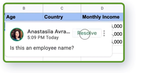Railsware is happy to share our best findings and approaches with readers, as well as our YouTube channel viewers. As a product development studio, we work with different business aspects from product development and design to marketing and analytics. More interesting insights are ahead, so stay with us to learn different useful things.