Google Sheets provides you with enormous opportunities to work with both numerical and verbal data. The thing is to know how to use this tool properly. Recently, we introduced a Google Sheets tutorial for beginners, so you could get familiar with the intricacies of the tool. Today, we’ll focus on data validation in GSheets. If you prefer watching than reading, check out the YouTube version of this tutorial.

Why you need data validation

The spreadsheet you’re working with must not contain incorrect data. This is dead weight on the efficiency of analytics. And that’s why you need to validate data. This process is essential to ensure your data is accurate and correct. When it comes to validating values in Google Sheets, there is a great function called Data Validation. It lets you set specific rules to assign values in a spreadsheet. Now, we’ll discover how it works in practice.

How to validate data in Google Sheets

We need a hands-on example to delve into this. Let’s take the payments database we often use in other GSheets videos. You can also get a personal copy of the Google Sheets practice file with Data Validation task to exercise with. Alternatively, you can import this data set using the following formula:

=QUERY(IMPORTRANGE(“https://docs.google.com/spreadsheets/d/1PIBARI0hgxzFQpNz_-KMxQ51oPRxUwd2w1Rx0nCUyDE/edit#gid=2047613745″,”Data Validation Basic!A:H”),“select *”)

Learn more about the combination of QUERY + IMPORTRANGE functions in Google Sheets.

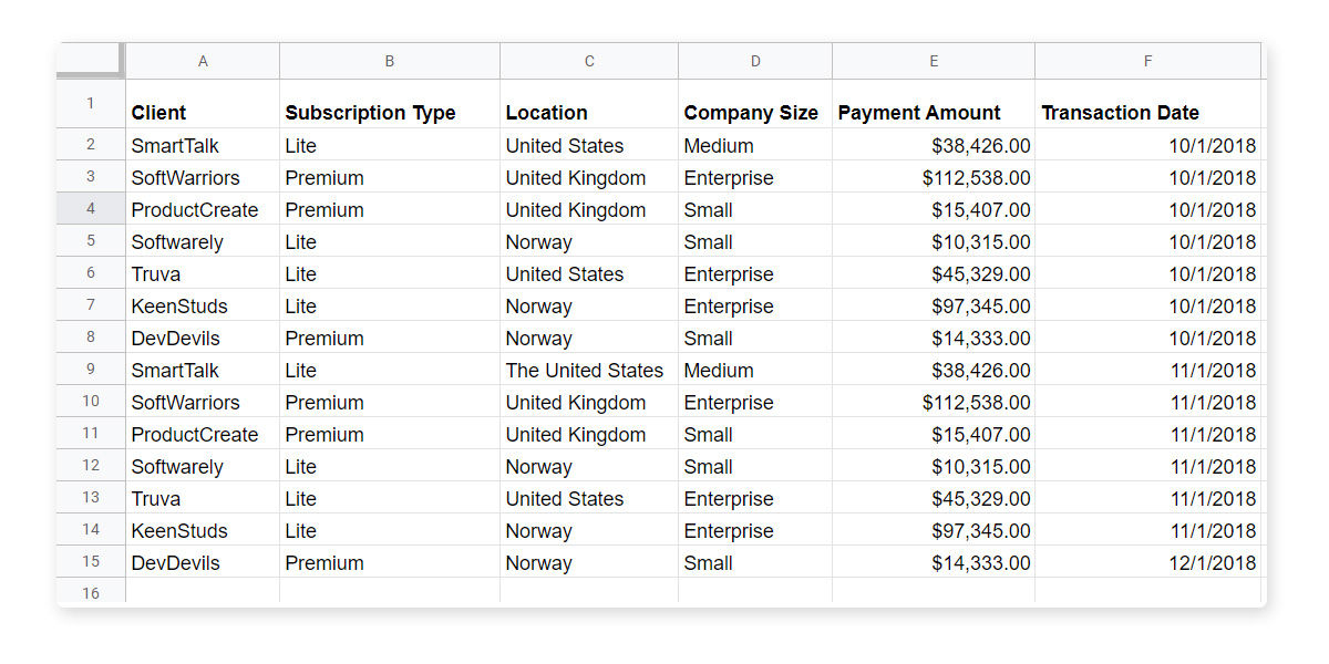
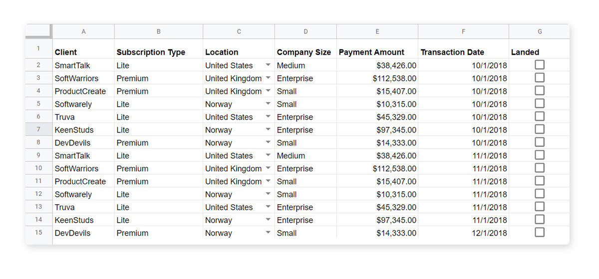
Here we have several data criteria:

• Names of clients
• Subscription type
• Location
• Company size
• Payment amounts
• Transaction date

The main thing to be done is to make sure that your data is accurate. This includes, for example, that the US clients have “United States” as their location. Meanwhile, such options as “The United States”, “US” or “USA” are inaccurate. And this is where the Data Validation function helps a lot.

Data validation using List of items

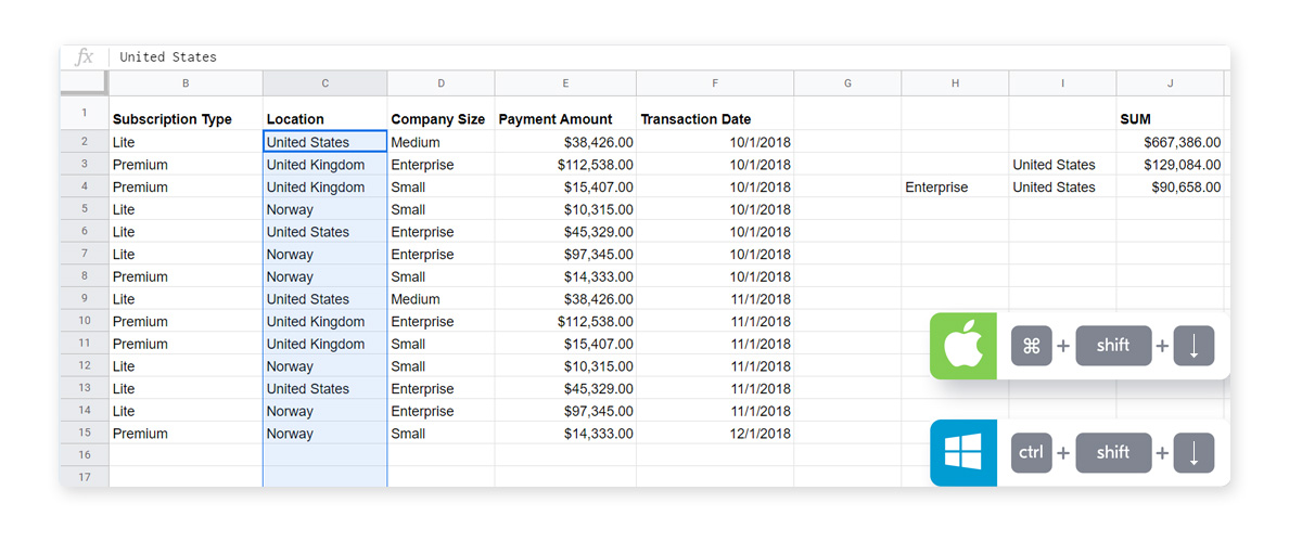
First of all, you need to select the dataset to be validated. We use the location column as an example. Since the first cell is a header, you need to start from C2. For Mac, click on C2 and then Command+Shift+Down. This selects all the cells in the column that contain values. It is better to select the whole column in case additional data appears. So, press Command+Shift+Down once more.

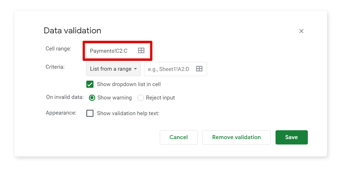
Then go to the menu: Data -> Data Validation, or you can right click and find Data Validation in the bottom. You can type in the Cell range manually here as well. To select the whole column starting from C2, type C2:C.

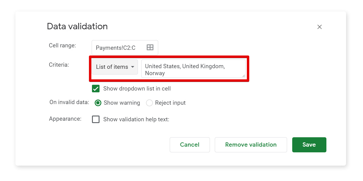
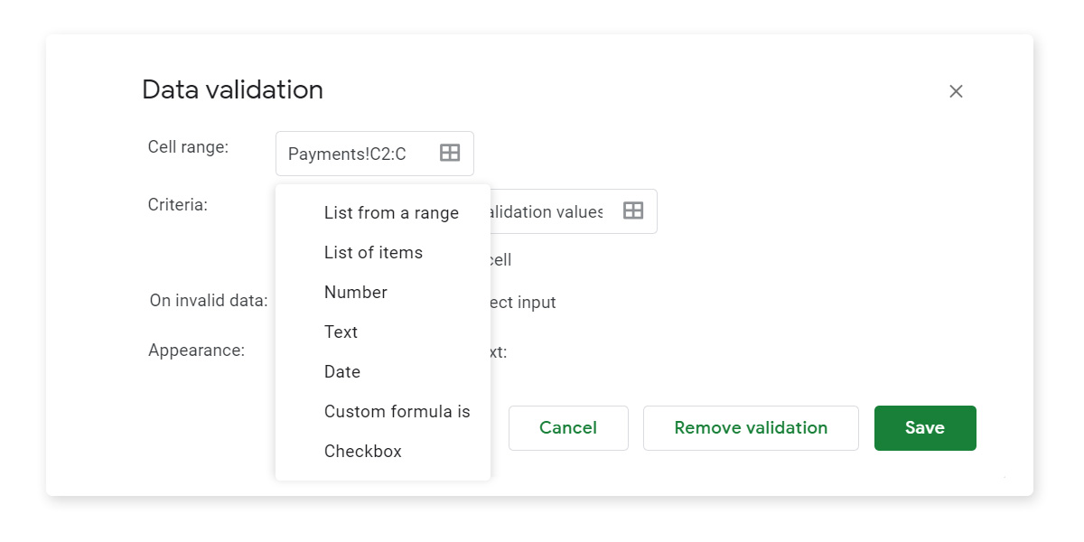
Now you need to define Criteria to fit. Let’s imagine you sell your services in three countries only: United States, United Kingdom, and Norway. If your range is fixed and won’t change often, choose the List of items option and type in all the items separated by commas. Remember that you have to use the correct letter case and no extra spaces. Press Save.

Now all the locations should fit one of the items from our list. If any values don’t fit, they will get marked as invalid like this one: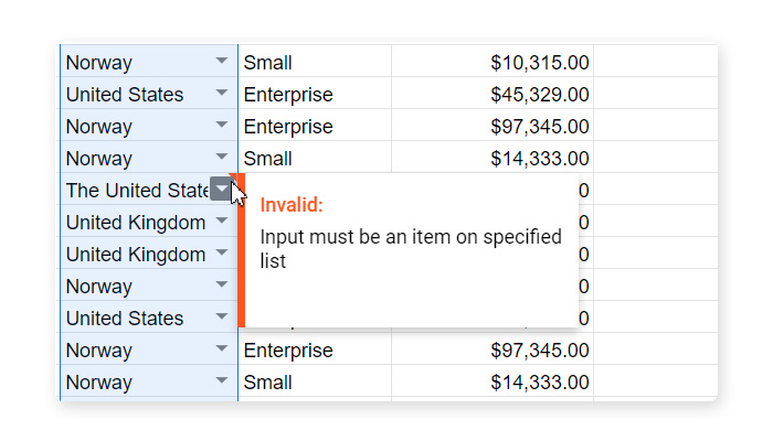

Data validation using List from a range

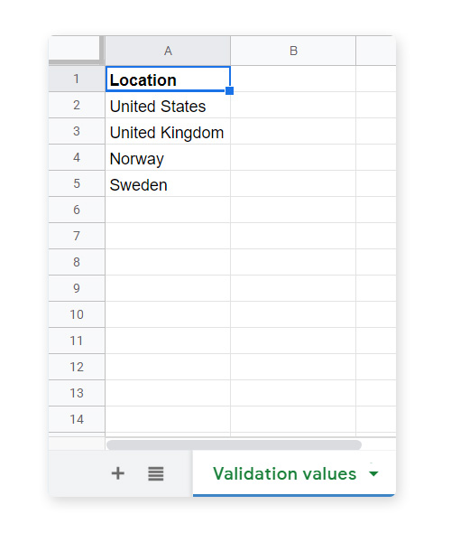
For example, you are expanding your business to new markets. So, your list of items is about to change. In this case, it is better to use the List from a range option. For this, select a separate column or create a new tab titled Validation values and select a column there. This column should contain the values to match for the locations from our dataset. Let’s call it Locations as well and add the following items:

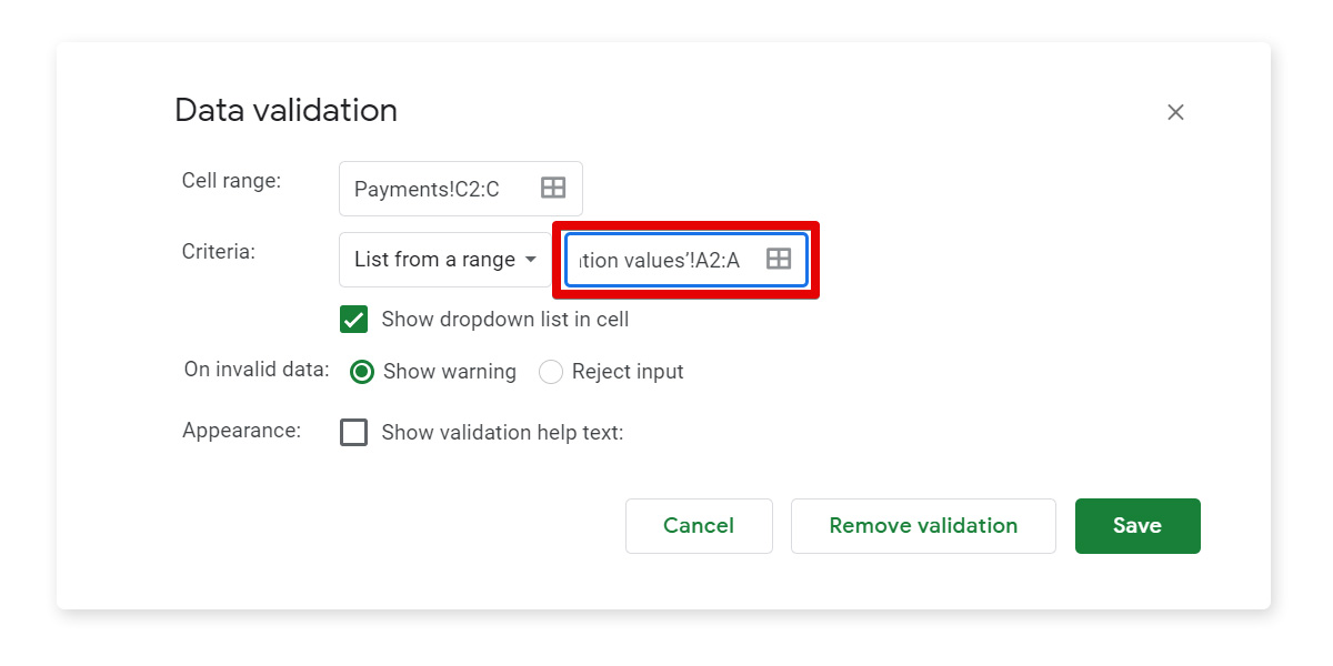
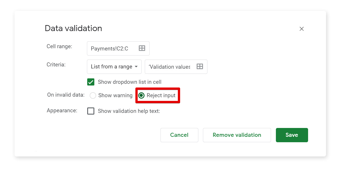
Go back to the Payments tab and select the locations column again. Or go directly to data validation and set a cell range there (C2:C). Now select the criteria – List from a range – and specify the range from the Validation values tab. The latter can be done by clicking the grid and manually selecting the range from the tab. The shorter option is to type ‘Validation values’!A2:A in the field. Press Save.

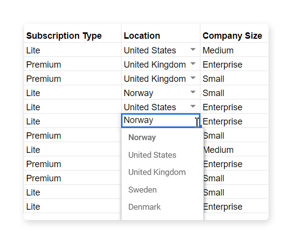
Now the locations should fit one of the values from our validation list. If you need to update your list from the Validation values tab, add new items to the column. For example, let’s add Denmark. It will appear in the drop-down list in the Locations column in the Payments tab. Do not add anything else to the validation column, as it will appear in the list too.

Other data validation options

Additionally, you can validate your data in a number of ways:

• if the values should match any specific number
• if the text should contain any specific words
• if the date in the range is before the deadline

Also you can apply custom formulas to data validation.

You may forbid inputting data that does not match the requirements you set. This will secure your dataset.

Google Sheets checkbox

Recently Google Sheets added a new feature to data validation. Now, you can create checklists and mark what was done/undone right in the spreadsheet. Imagine you need to mark the payments that have already landed on our bank account. Create a separate column called Landed. Go to data validation, select the cell range G2:G, and then pick the Checkbox option. Click Save.

Now you can mark which payments have already landed on your bank account. The Checkbox option lets you manage various processes in Google Sheets.

This was the introduction to data validation function in Google Sheets. This tool has a lot of quirks the Railsware team is going to explore in more detail later. So, read our blog and subscribe to our YouTube channel to get more interesting insights.